Apache Iceberg Masterclass - Table of Contents
- What Are Table Formats and Why Were They Needed?
- The Metadata Structure of Modern Table Formats
- Performance and Apache Iceberg’s Metadata
- Partition Evolution: Change Your Partitioning Without Rewriting Data
- Hidden Partitioning: How Iceberg Eliminates Accidental Full Table Scans
- Writing to an Apache Iceberg Table: How Commits and ACID Actually Work
- What Are Lakehouse Catalogs? The Role of Catalogs in Apache Iceberg
- When Catalogs Are Embedded in Storage
- How Data Lake Table Storage Degrades Over Time
- Maintaining Apache Iceberg Tables: Compaction, Expiry, and Cleanup
- Apache Iceberg Metadata Tables: Querying the Internals
- Using Apache Iceberg with Python and MPP Query Engines
- Approaches to Streaming Data into Apache Iceberg Tables
- Hands-On with Apache Iceberg Using Dremio Cloud
- Migrating to Apache Iceberg: Strategies for Every Source System
This is Part 5 of a 15-part Apache Iceberg Masterclass. Part 4 covered partition evolution. This article covers hidden partitioning, the feature that ensures users never need to know how their data is physically organized.
The most expensive mistake in data lake querying is the accidental full table scan: a query that reads every file because the user did not correctly reference the partition columns. In Hive, this happens constantly. In Iceberg, it is structurally impossible because users never reference partition columns at all.
The Accidental Full Scan Problem
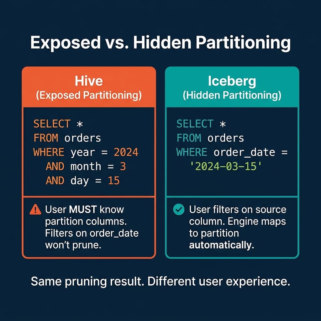
In Hive, a table partitioned by year, month, and day requires queries to filter on those exact columns:
-- Hive: This prunes correctly
SELECT * FROM orders WHERE year = 2024 AND month = 3 AND day = 15

-- Hive: This scans EVERYTHING (no pruning)
SELECT * FROM orders WHERE order_date = '2024-03-15'
The second query reads every partition because Hive does not know that order_date maps to the year, month, and day partition columns. There is no error, no warning. The query simply runs 100x slower than it should.
This happens because Hive partitioning is “exposed.” The physical partition columns (year, month, day) are separate from the source column (order_date). Users must understand this mapping and construct their filters accordingly.
How Iceberg Hides Partitioning
Iceberg flips this model. Users filter on the source column (order_date), and the engine automatically maps the filter to the partition values using transform functions.
-- Iceberg: This prunes correctly. Always.
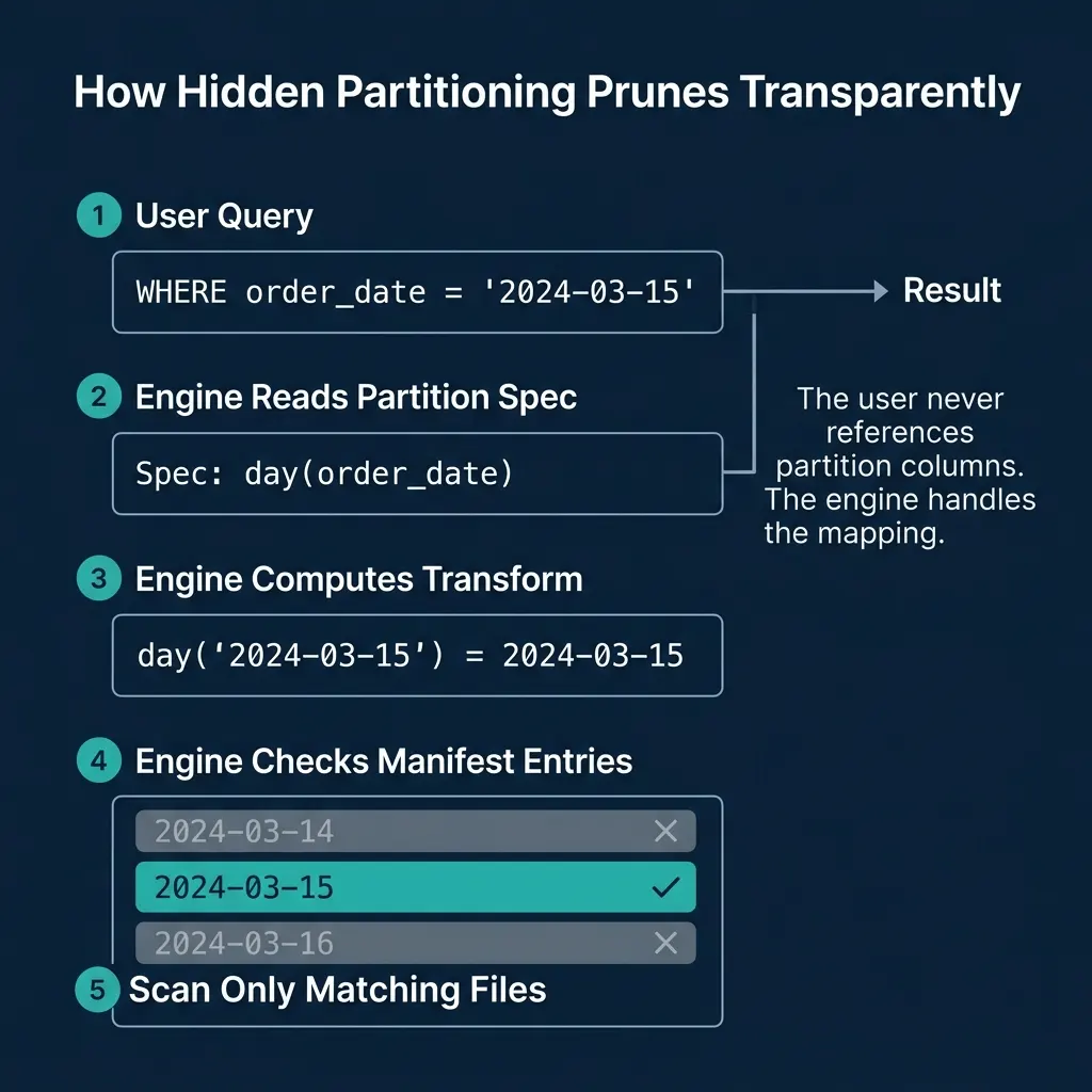
SELECT * FROM orders WHERE order_date = '2024-03-15'The table’s partition spec declares: PARTITIONED BY (day(order_date)). When the engine processes this query, it:
- Reads the partition spec from the table metadata
- Applies the
day()transform to the filter value:day('2024-03-15')=2024-03-15 - Checks manifest entries for files with matching partition values
- Skips every file whose partition value is not
2024-03-15
The user writes natural SQL against the source columns. The engine handles the physical-to-logical mapping. This is why it is called “hidden” partitioning: the partition structure is invisible to the user.
The Six Transform Functions
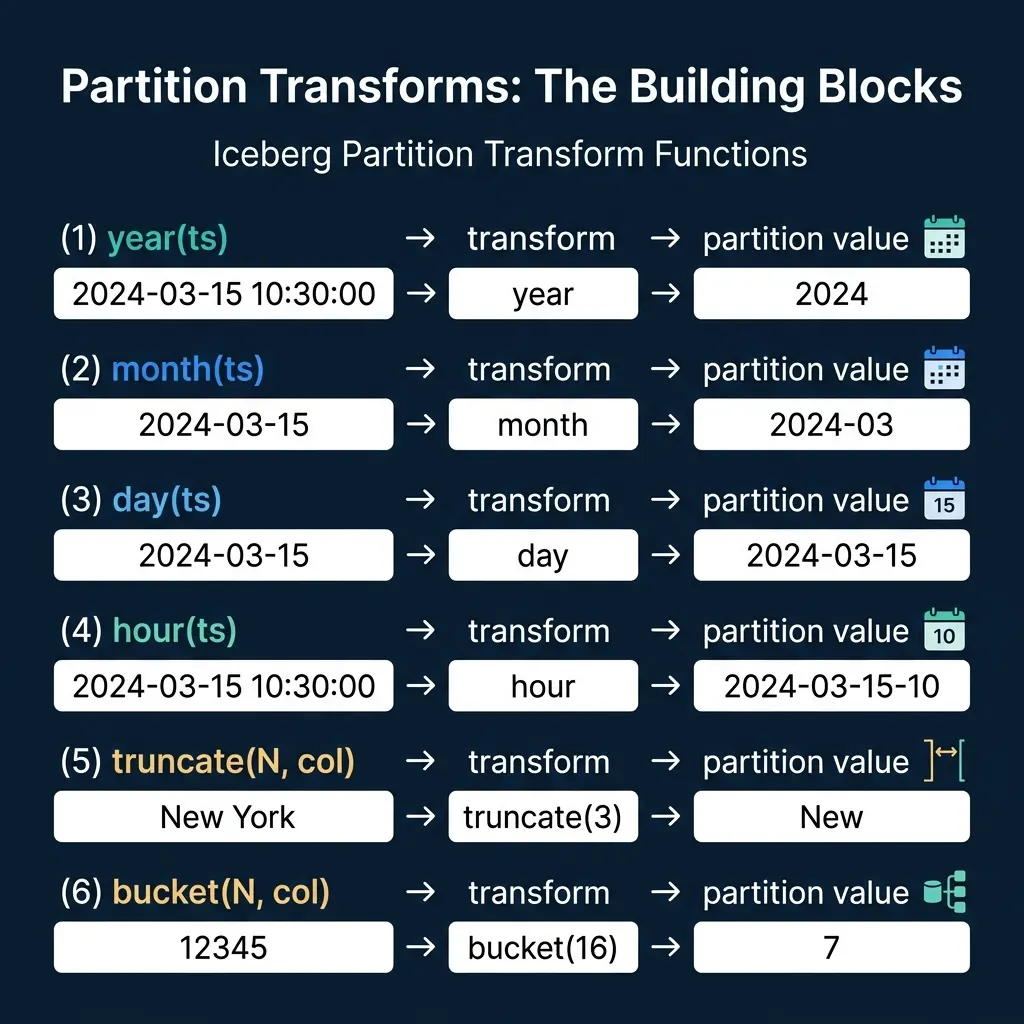
Iceberg defines six partition transforms that map source column values to partition values:
Temporal Transforms
| Transform | Input | Output | Use Case |
|---|---|---|---|
year(ts) | 2024-03-15 10:30:00 | 2024 | Low-volume tables, yearly reporting |
month(ts) | 2024-03-15 10:30:00 | 2024-03 | Medium-volume tables, monthly queries |
day(ts) | 2024-03-15 10:30:00 | 2024-03-15 | High-volume tables, daily queries |
hour(ts) | 2024-03-15 10:30:00 | 2024-03-15-10 | Very high-volume streaming data |
The temporal transforms are hierarchical. If a table is partitioned by day(ts) and a user filters WHERE ts >= '2024-03-01' AND ts < '2024-04-01', the engine recognizes this as a range of days and prunes to only the 31 matching partitions. Engines like Dremio handle this mapping automatically for equality, range, and IN-list predicates.
Value Transforms
| Transform | Input | Output | Use Case |
|---|---|---|---|
truncate(N, col) | 'New York' (N=3) | 'New' | Grouping strings by prefix |
bucket(N, col) | 12345 (N=16) | 7 | Even distribution of high-cardinality columns |
truncate(N, col) takes the first N characters of a string (or truncates a number to a width). This is useful when you want to group data by a string prefix without creating one partition per unique value.
bucket(N, col) applies a hash function and mod N to produce a bucket number from 0 to N-1. This distributes data evenly across a fixed number of buckets, regardless of the column’s value distribution. It is the go-to transform for high-cardinality columns like user_id or order_id where identity partitioning would create millions of tiny partitions.
The Identity Transform
The identity transform (identity(col)) uses the raw column value as the partition value. This is equivalent to Hive-style partitioning, but the column is still “hidden” because the engine handles the mapping. It is useful for low-cardinality columns like region or status where each unique value should be its own partition.
How Pruning Works Under the Hood
The pruning process works in three phases:
Phase 1: Predicate translation. The engine examines each WHERE clause predicate and checks if the filtered column is part of the partition spec. If order_date is the source column for day(order_date), the engine can translate order_date = '2024-03-15' into a partition filter.
Phase 2: Manifest list evaluation. The manifest list stores partition value ranges per manifest. The engine checks if each manifest’s range includes the target partition value. Manifests whose range does not overlap are skipped entirely.
Phase 3: Manifest entry evaluation. For each surviving manifest, the engine checks individual file entries. Only files whose partition value matches 2024-03-15 are included in the scan plan.
This is the same pruning cascade described in Part 3, but now the partition values were derived automatically from the user’s filter on a source column.
Choosing the Right Transform
The choice of partition transform depends on data volume and query patterns:
| Scenario | Recommended Transform | Rationale |
|---|---|---|
| 10 GB/day of event data | day(event_time) | Each day is one partition (~10 GB), well-sized files |
| 1 TB/day of event data | hour(event_time) | Each hour is ~42 GB, prevents oversized partitions |
| 500 MB/month of reports | month(report_date) | Monthly partitions keep file counts manageable |
| User-level data, 10M users | bucket(64, user_id) | Even distribution, avoids millions of tiny partitions |
| Region-based data, 5 regions | identity(region) | Only 5 partitions, each meaningfully distinct |
The goal is to create partitions that are large enough to contain optimally-sized files (128-512 MB each) but small enough that partition pruning eliminates most files for typical queries.
Over-partitioning (too many small partitions) creates the small file problem: thousands of tiny files that bloat metadata and slow query planning. Under-partitioning (too few large partitions) reduces pruning effectiveness because each partition contains too much data.
Combining Transforms
Iceberg supports multi-column partition specs:
CREATE TABLE events (
  event_id BIGINT,
  event_time TIMESTAMP,
  user_id BIGINT,
  event_type STRING
) PARTITIONED BY (day(event_time), bucket(32, user_id))
This creates a two-dimensional partition space: each combination of day and user bucket is a separate partition. Queries filtering on event_time get day-level pruning. Queries filtering on user_id get bucket-level pruning. Queries filtering on both get pruning from both dimensions.
Dremio supports all Iceberg transform functions and automatically applies pruning for any combination of partition columns in the query’s WHERE clause.
Why This Matters for Teams
Hidden partitioning changes the operational model for data teams:
Data engineers define the partition strategy once in the table’s partition spec. They can change it later through partition evolution without breaking anything.
Analysts and data scientists write natural SQL against the business columns they understand. They never need to know whether the table is partitioned by day, month, or bucket. Their queries are automatically optimized.
BI tools and dashboards connect to Iceberg tables and issue standard SQL. The tools do not need to understand Iceberg’s partitioning; the engine handles the optimization. This is why hidden partitioning is essential for self-service analytics platforms like Dremio.
The net result: no accidental full table scans, no partition-aware query patterns required from users, and the ability to change the physical layout without impacting any downstream consumer. Part 6 covers what happens when data is written to an Iceberg table.
Books to Go Deeper
- Architecting the Apache Iceberg Lakehouse by Alex Merced (Manning)
- Lakehouses with Apache Iceberg: Agentic Hands-on by Alex Merced
- Constructing Context: Semantics, Agents, and Embeddings by Alex Merced
- Apache Iceberg & Agentic AI: Connecting Structured Data by Alex Merced
- Open Source Lakehouse: Architecting Analytical Systems by Alex Merced